Run STitch3D on the DLPFC dataset
In this tutorial, we show STitch3D’s analysis of the human dorsolateral prefrontal cortex (DLPFC) dataset.
The spatial transcriptomics DLPFC data are publicly available at https://github.com/LieberInstitute/spatialLIBD. The DLPFC dataset profiled by 10x Genomics Chromium platform is available at https://www.ncbi.nlm.nih.gov/geo/query/acc.cgi?acc=GSE144136.
Import packages
[1]:
import pandas as pd
import numpy as np
import scanpy as sc
import anndata as ad
import scipy.io
import matplotlib.pyplot as plt
import os
import sys

import STitch3D

import warnings
warnings.filterwarnings("ignore")

os.environ["CUDA_VISIBLE_DEVICES"] = "0"
Preprocessing
Load datasets
Load single-cell reference dataset:
[2]:
mat = scipy.io.mmread("./data/snRNAseq_brain/GSE144136_GeneBarcodeMatrix_Annotated.mtx")
meta = pd.read_csv("./data/snRNAseq_brain/GSE144136_CellNames.csv", index_col=0)
meta.index = meta.x.values
group = [i.split('.')[1].split('_')[0] for i in list(meta.x.values)]
condition = [i.split('.')[1].split('_')[1] for i in list(meta.x.values)]
celltype = [i.split('.')[0] for i in list(meta.x.values)]
meta["group"] = group
meta["condition"] = condition
meta["celltype"] = celltype
genename = pd.read_csv("./data/snRNAseq_brain/GSE144136_GeneNames.csv", index_col=0)
genename.index = genename.x.values
adata_ref = ad.AnnData(X=mat.tocsr().T)
adata_ref.obs = meta
adata_ref.var = genename
adata_ref = adata_ref[adata_ref.obs.condition.values.astype(str)=="Control", :]
Load spatial transcriptomics datasets:
[3]:
#spatial data
anno_df = pd.read_csv('./data/spatialLIBD/barcode_level_layer_map.tsv', sep='\t', header=None)

slice_idx = [151673, 151674, 151675, 151676]

adata_st1 = sc.read_visium(path="./data/spatialLIBD/%d" % slice_idx[0],
                          count_file="%d_filtered_feature_bc_matrix.h5" % slice_idx[0])
anno_df1 = anno_df.iloc[anno_df[1].values.astype(str) == str(slice_idx[0])]
anno_df1.columns = ["barcode", "slice_id", "layer"]
anno_df1.index = anno_df1['barcode']
adata_st1.obs = adata_st1.obs.join(anno_df1, how="left")
adata_st1 = adata_st1[adata_st1.obs['layer'].notna()]

adata_st2 = sc.read_visium(path="./data/spatialLIBD/%d" % slice_idx[1],
                          count_file="%d_filtered_feature_bc_matrix.h5" % slice_idx[1])
anno_df2 = anno_df.iloc[anno_df[1].values.astype(str) == str(slice_idx[1])]
anno_df2.columns = ["barcode", "slice_id", "layer"]
anno_df2.index = anno_df2['barcode']
adata_st2.obs = adata_st2.obs.join(anno_df2, how="left")
adata_st2 = adata_st2[adata_st2.obs['layer'].notna()]

adata_st3 = sc.read_visium(path="./data/spatialLIBD/%d" % slice_idx[2],
                          count_file="%d_filtered_feature_bc_matrix.h5" % slice_idx[2])
anno_df3 = anno_df.iloc[anno_df[1].values.astype(str) == str(slice_idx[2])]
anno_df3.columns = ["barcode", "slice_id", "layer"]
anno_df3.index = anno_df3['barcode']
adata_st3.obs = adata_st3.obs.join(anno_df3, how="left")
adata_st3 = adata_st3[adata_st3.obs['layer'].notna()]

adata_st4 = sc.read_visium(path="./data/spatialLIBD/%d" % slice_idx[3],
                          count_file="%d_filtered_feature_bc_matrix.h5" % slice_idx[3])
anno_df4 = anno_df.iloc[anno_df[1].values.astype(str) == str(slice_idx[3])]
anno_df4.columns = ["barcode", "slice_id", "layer"]
anno_df4.index = anno_df4['barcode']
adata_st4.obs = adata_st4.obs.join(anno_df4, how="left")
adata_st4 = adata_st4[adata_st4.obs['layer'].notna()]
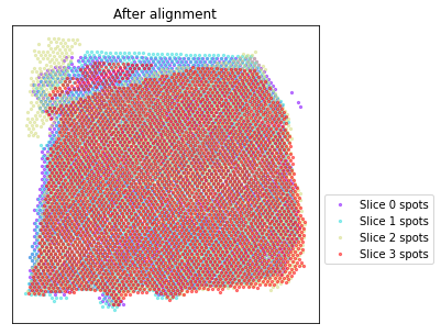
Alignment of ST tissue slices
[4]:
adata_st_list_raw = [adata_st1, adata_st2, adata_st3, adata_st4]
adata_st_list = STitch3D.utils.align_spots(adata_st_list_raw, plot=True)

Using the Iterative Closest Point algorithm for alignemnt.
Detecting edges...
Aligning edges...
Selecting highly variable genes and building 3D spatial graph
[5]:
celltype_list_use = ['Astros_1', 'Astros_2', 'Astros_3', 'Endo', 'Micro/Macro',
                     'Oligos_1', 'Oligos_2', 'Oligos_3',
                     'Ex_1_L5_6', 'Ex_2_L5', 'Ex_3_L4_5', 'Ex_4_L_6', 'Ex_5_L5',
                     'Ex_6_L4_6', 'Ex_7_L4_6', 'Ex_8_L5_6', 'Ex_9_L5_6', 'Ex_10_L2_4']

adata_st, adata_basis = STitch3D.utils.preprocess(adata_st_list,
                                                  adata_ref,
                                                  celltype_ref=celltype_list_use,
                                                  sample_col="group",
                                                  slice_dist_micron=[10., 300., 10.],
                                                  n_hvg_group=500)
Finding highly variable genes...
4558 highly variable genes selected.
Calculate basis for deconvolution...
1 batches are used for computing the basis vector of cell type <Astros_1>.
17 batches are used for computing the basis vector of cell type <Astros_2>.
14 batches are used for computing the basis vector of cell type <Astros_3>.
17 batches are used for computing the basis vector of cell type <Endo>.
17 batches are used for computing the basis vector of cell type <Ex_10_L2_4>.
15 batches are used for computing the basis vector of cell type <Ex_1_L5_6>.
15 batches are used for computing the basis vector of cell type <Ex_2_L5>.
17 batches are used for computing the basis vector of cell type <Ex_3_L4_5>.
14 batches are used for computing the basis vector of cell type <Ex_4_L_6>.
17 batches are used for computing the basis vector of cell type <Ex_5_L5>.
16 batches are used for computing the basis vector of cell type <Ex_6_L4_6>.
16 batches are used for computing the basis vector of cell type <Ex_7_L4_6>.
15 batches are used for computing the basis vector of cell type <Ex_8_L5_6>.
13 batches are used for computing the basis vector of cell type <Ex_9_L5_6>.
16 batches are used for computing the basis vector of cell type <Micro/Macro>.
8 batches are used for computing the basis vector of cell type <Oligos_1>.
4 batches are used for computing the basis vector of cell type <Oligos_2>.
16 batches are used for computing the basis vector of cell type <Oligos_3>.
Preprocess ST data...
Start building a graph...
Radius for graph connection is 150.7000.
9.8415 neighbors per cell on average.
Running STitch3D model
[6]:
model = STitch3D.model.Model(adata_st, adata_basis)

model.train()
0%| | 2/20000 [00:00<1:29:35, 3.72it/s]
Step: 0, Loss: 2438.9314, d_loss: 2433.3323, f_loss: 55.9906
10%|█ | 2002/20000 [06:09<55:06, 5.44it/s]
Step: 2000, Loss: 745.4474, d_loss: 742.1439, f_loss: 33.0354
20%|██ | 4002/20000 [12:20<49:15, 5.41it/s]
Step: 4000, Loss: 706.4982, d_loss: 703.2151, f_loss: 32.8299
30%|███ | 6002/20000 [18:31<42:47, 5.45it/s]
Step: 6000, Loss: 697.4716, d_loss: 694.2027, f_loss: 32.6885
40%|████ | 8002/20000 [24:43<37:00, 5.40it/s]
Step: 8000, Loss: 693.6924, d_loss: 690.4269, f_loss: 32.6556
50%|█████ | 10002/20000 [30:55<31:00, 5.37it/s]
Step: 10000, Loss: 692.3774, d_loss: 689.1337, f_loss: 32.4372
60%|██████ | 12002/20000 [37:08<24:44, 5.39it/s]
Step: 12000, Loss: 693.6156, d_loss: 690.3403, f_loss: 32.7528
70%|███████ | 14002/20000 [43:20<18:21, 5.45it/s]
Step: 14000, Loss: 691.1208, d_loss: 687.8664, f_loss: 32.5445
80%|████████ | 16002/20000 [49:31<12:17, 5.42it/s]
Step: 16000, Loss: 690.3745, d_loss: 687.1446, f_loss: 32.2987
90%|█████████ | 18002/20000 [55:43<06:06, 5.45it/s]
Step: 18000, Loss: 689.8022, d_loss: 686.5756, f_loss: 32.2657
100%|██████████| 20000/20000 [1:01:54<00:00, 5.38it/s]
Saving STitch3D results
[7]:
save_path = "./results_DLPFC"
result = model.eval(adata_st_list_raw, save=True, output_path=save_path)
Visualizing results in 2D
STitch3D’s learned representations of spots in all slices are restored in “model.adata_st.obsm[‘latent’]”, which are used for spatial domain identification.
[8]:
from sklearn.mixture import GaussianMixture

np.random.seed(1234)
gm = GaussianMixture(n_components=7, covariance_type='tied', init_params='kmeans')
y = gm.fit_predict(model.adata_st.obsm['latent'], y=None)
model.adata_st.obs["GM"] = y
model.adata_st.obs["GM"].to_csv(os.path.join(save_path, "clustering_result.csv"))

# Restoring clustering labels to result
order = [2,4,6,0,3,5,1] # reordering cluster labels
model.adata_st.obs["Cluster"] = [order[label] for label in model.adata_st.obs["GM"].values]
for i in range(len(result)):
    result[i].obs["GM"] = model.adata_st.obs.loc[result[i].obs_names, ]["GM"]
    result[i].obs["Cluster"] = model.adata_st.obs.loc[result[i].obs_names, ]["Cluster"]
Plotting spatial domains:
[9]:
for i, adata_st_i in enumerate(result):
    print("Slice %d spatial domain detection result:" % slice_idx[i])
    sc.pl.spatial(adata_st_i, img_key="lowres", color="Cluster", color_map="cividis", size=1.)
Slice 151673 spatial domain detection result:

Slice 151674 spatial domain detection result:

Slice 151675 spatial domain detection result:

Slice 151676 spatial domain detection result:

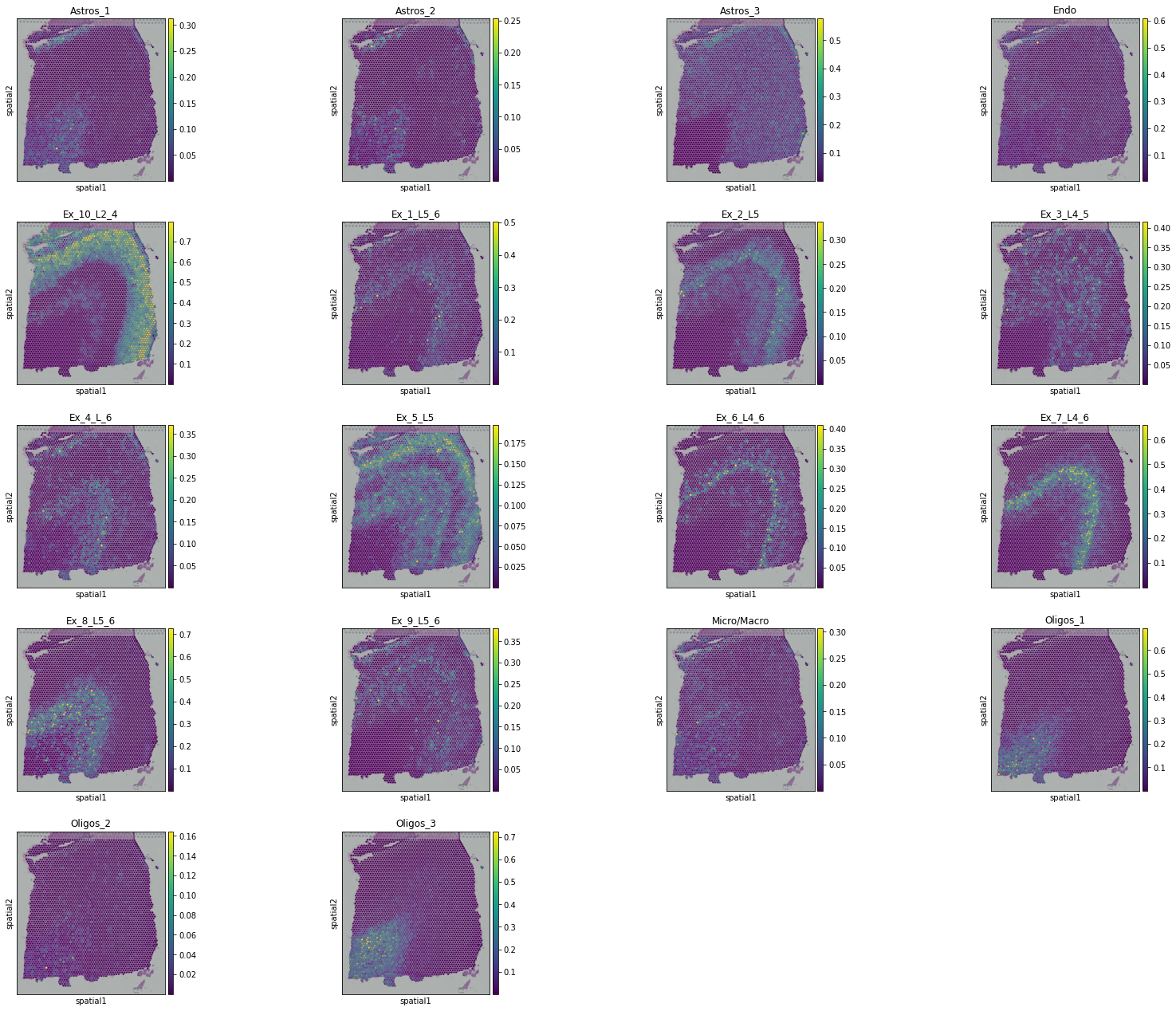
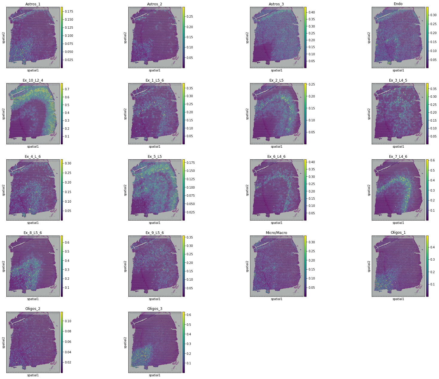
Plotting cell-type proportions:
[10]:
for i, adata_st_i in enumerate(result):
    print("Slice %d cell-type deconvolution result:" % slice_idx[i])
    sc.pl.spatial(adata_st_i, img_key="lowres", color=list(adata_basis.obs.index), size=1.)
Slice 151673 cell-type deconvolution result:
Slice 151674 cell-type deconvolution result:
Slice 151675 cell-type deconvolution result:

Slice 151676 cell-type deconvolution result:

Plotting UMAP:
[11]:
import umap

reducer = umap.UMAP(n_neighbors=30,
                    n_components=2,
                    metric="correlation",
                    n_epochs=None,
                    learning_rate=1.0,
                    min_dist=0.3,
                    spread=1.0,
                    set_op_mix_ratio=1.0,
                    local_connectivity=1,
                    repulsion_strength=1,
                    negative_sample_rate=5,
                    a=None,
                    b=None,
                    random_state=1234,
                    metric_kwds=None,
                    angular_rp_forest=False,
                    verbose=True)

embedding = reducer.fit_transform(model.adata_st.obsm['latent'])

n_spots = embedding.shape[0]
size = 120000 / n_spots
UMAP(angular_rp_forest=True, dens_frac=0.0, dens_lambda=0.0,
     local_connectivity=1, metric='correlation', min_dist=0.3, n_neighbors=30,
     random_state=1234, repulsion_strength=1, verbose=True)
Construct fuzzy simplicial set
Thu Feb  2 15:11:04 2023 Finding Nearest Neighbors
Thu Feb  2 15:11:04 2023 Building RP forest with 11 trees
Thu Feb  2 15:11:05 2023 NN descent for 14 iterations
         1  /  14
         2  /  14
         3  /  14
        Stopping threshold met -- exiting after 3 iterations
Thu Feb  2 15:11:17 2023 Finished Nearest Neighbor Search
Thu Feb  2 15:11:20 2023 Construct embedding
        completed  0  /  200 epochs
        completed  20  /  200 epochs
        completed  40  /  200 epochs
        completed  60  /  200 epochs
        completed  80  /  200 epochs
        completed  100  /  200 epochs
        completed  120  /  200 epochs
        completed  140  /  200 epochs
        completed  160  /  200 epochs
        completed  180  /  200 epochs
Thu Feb  2 15:11:35 2023 Finished embedding
Obtaining spatial trajectory with PAGA (https://scanpy.readthedocs.io/en/stable/generated/scanpy.tl.paga.html).
[12]:
model.adata_st.obsm["X_umap"] = embedding
sc.pp.neighbors(model.adata_st, use_rep='latent')
sc.tl.paga(model.adata_st, groups='layer')
[13]:
from sklearn import preprocessing
from matplotlib.colors import ListedColormap

le_slice = preprocessing.LabelEncoder()
label_slice = le_slice.fit_transform(model.adata_st.obs['slice_id'])

le_layer = preprocessing.LabelEncoder()
label_layer = le_layer.fit_transform(model.adata_st.obs['layer'])

np.random.seed(1234)
order = np.arange(n_spots)
np.random.shuffle(order)

f = plt.figure(figsize=(45,10))

ax1 = f.add_subplot(1,4,1)
scatter1 = ax1.scatter(embedding[order, 0], embedding[order, 1],
                       s=size, c=label_slice[order], cmap='coolwarm')
ax1.set_title("Slice", fontsize=40)
ax1.tick_params(axis='both',bottom=False, top=False, left=False, right=False, labelleft=False, labelbottom=False, grid_alpha=0)

l1 = ax1.legend(handles=scatter1.legend_elements()[0],
                labels=["Slice %d" % i for i in slice_idx],
                loc="upper left", bbox_to_anchor=(0., 0.),
                markerscale=3., title_fontsize=45, fontsize=30, frameon=False, ncol=1)
l1._legend_box.align = "left"


ax2 = f.add_subplot(1,4,2)
scatter2 = ax2.scatter(embedding[order, 0], embedding[order, 1],
                       s=size, c=model.adata_st.obs['Cluster'][order], cmap='cividis')
ax2.set_title("Cluster", fontsize=40)
ax2.tick_params(axis='both',bottom=False, top=False, left=False, right=False, labelleft=False, labelbottom=False, grid_alpha=0)

l2 = ax2.legend(handles=scatter2.legend_elements()[0],
                labels=["Cluster %d" % i for i in range(1, 8)],
                loc="upper left", bbox_to_anchor=(0., 0.),
                markerscale=3., title_fontsize=45, fontsize=30, frameon=False, ncol=2)

l2._legend_box.align = "left"

ax3 = f.add_subplot(1,4,3)
scatter3 = ax3.scatter(embedding[order, 0], embedding[order, 1],
                       s=size, c=label_layer[order], cmap=ListedColormap(["#1f77b4", "#ff7f0e", "#2ca02c", "#d62728", "#9467bd", "#8c564b", "#e377c2"]))
ax3.set_title("Layer annotation", fontsize=40)
ax3.tick_params(axis='both',bottom=False, top=False, left=False, right=False, labelleft=False, labelbottom=False, grid_alpha=0)

l3 = ax3.legend(handles=scatter3.legend_elements()[0],
                labels=sorted(set(adata_st.obs['layer'].values)),
                loc="upper left", bbox_to_anchor=(0., 0.),
                markerscale=3., title_fontsize=45, fontsize=30, frameon=False, ncol=2)

l3._legend_box.align = "left"

ax4 = f.add_subplot(1,4,4)
ax4.set_title("Trajectory", fontsize=40)
ax4.tick_params(axis='both',bottom=False, top=False, left=False, right=False, labelleft=False, labelbottom=False, grid_alpha=0)
ax4.set_xlim(ax3.get_xlim())
ax4.set_ylim(ax3.get_ylim())

pos = []
for layer in ["L1", "L2", "L3", "L4", "L5", "L6", "WM"]:
    center = np.mean(embedding[model.adata_st.obs['layer'].values.astype(str)==layer, :], axis=0)
    pos.append(center)

sc.pl.paga(adata_st, pos=np.array(pos), node_size_scale=20, edge_width_scale=5, fontsize=20, fontoutline=3, ax=ax4)

f.subplots_adjust(hspace=.1, wspace=.1)
plt.show()
