Run STitch3D on the Drosophila embryo dataset

In this tutorial, we show STitch3D’s analysis of the Drosophila embryo dataset.

The Drosophila embryo Stereo-seq dataset is publicly available at (https://db.cngb.org/stomics/flysta3d/download.html. The Drosophila embryo sci-RNA-seq dataset is publicly available at https://www.ncbi.nlm.nih.gov/geo/query/acc.cgi?acc=GSE190149.

Import packages

import pandas as pd
import numpy as np
import scanpy as sc
import anndata as ad
from scipy.io import mmread
import os
import sys

import STitch3D

import warnings
warnings.filterwarnings("ignore")

os.environ["CUDA_VISIBLE_DEVICES"] = "5"

Preprocessing

Load datasets

Load single-cell reference dataset:

ref_count = mmread("./data/Calderon_2022/GSE190147_scirnaseq_gene_matrix.mtx")
ref_row = pd.read_csv("./data/Calderon_2022/GSE190147_scirnaseq_gene_matrix.rows.txt",
                      header=None, index_col=0)
ref_col = pd.read_csv("./data/Calderon_2022/GSE190147_scirnaseq_gene_matrix.columns.txt",
                      index_col=0, sep='\t')

adata_ref_raw = ad.AnnData(X=ref_count.tocsr().T)
adata_ref_raw.obs = ref_col
adata_ref_raw.var.index = [str(i) for i in list(ref_row.index)]

adata_ref = ad.AnnData(X=adata_ref_raw.X)
adata_ref.obs = adata_ref_raw.obs
adata_ref.var = adata_ref_raw.var

adata_ref = adata_ref[adata_ref.obs['time'] == 'hrs_16_20']
adata_ref.obs.rename(columns = {'exp': 'exp_idx'}, inplace = True)

clust = pd.read_csv("./data/Calderon_2022/seurat_clust_1620.txt", sep=" ")
clust.index = clust.barcode.values.astype(str)
clust = clust.loc[adata_ref.obs.index, :]
adata_ref.obs["seurat_clust"] = clust.clust.values.astype(str)

#transfer clusters to cell type annotations
anno_table = pd.read_csv("./data/Calderon_2022/cluster_anno_table.csv")

adata_ref.obs['celltype'] = adata_ref.obs['seurat_clust'].values.astype(str)
for i in range(anno_table.shape[0]):
    adata_ref.obs['celltype'] = adata_ref.obs['celltype'].replace(anno_table["cluster"][i].astype(str),
                                                                  anno_table["annotation"][i])

adata_ref = adata_ref[(adata_ref.obs['celltype'] != "lowq") & (adata_ref.obs['celltype'] != "unk"), :]
clust = clust.loc[adata_ref.obs.index, :]

#plot umap
adata_ref_umap = adata_ref.copy()
hvg_num = 2000
sc.pp.highly_variable_genes(adata_ref_umap, flavor='seurat_v3', n_top_genes=hvg_num)
sc.pp.normalize_total(adata_ref_umap, target_sum=1e4)
sc.pp.log1p(adata_ref_umap)
sc.pp.scale(adata_ref_umap, max_value=10)
sc.tl.pca(adata_ref_umap, n_comps=30, svd_solver='arpack')
sc.pp.neighbors(adata_ref_umap, n_pcs=30)
sc.tl.umap(adata_ref_umap)
sc.pl.umap(adata_ref_umap, color=['celltype'])

Load spatial transcriptomics datasets:

#spatial data
adata_st_raw = sc.read_h5ad("./data/stereoseq_data/E16-18h_a_count_normal_stereoseq.h5ad")
adata_st_raw.X = adata_st_raw.layers['raw_counts']

slice_all = sorted(list(set(adata_st_raw.obs['slice_ID'].values)))[:-1]

adata_st_list_raw = []
for slice_id in slice_all:
    adata_st_i = adata_st_raw[adata_st_raw.obs['slice_ID'].values == slice_id]
    adata_st_i.obsm['spatial'] = np.concatenate((adata_st_i.obs['raw_x'].values.reshape(-1, 1),
                                                 adata_st_i.obs['raw_y'].values.reshape(-1, 1)), axis=1) / 20
    adata_st_i.obsm['loc_use'] = np.concatenate((adata_st_i.obs['raw_x'].values.reshape(-1, 1),
                                                 adata_st_i.obs['raw_y'].values.reshape(-1, 1)), axis=1) / 20
    adata_st_i.obsm['coor_3d'] = np.concatenate((adata_st_i.obs['new_x'].values.reshape(-1, 1),
                                                 adata_st_i.obs['new_y'].values.reshape(-1, 1),
                                                 adata_st_i.obs['new_z'].values.reshape(-1, 1)), axis=1)
    adata_st_i.obs['array_row'] = adata_st_i.obs['raw_y'].values
    adata_st_i.obs['array_col'] = adata_st_i.obs['raw_x'].values

    adata_st_list_raw.append(adata_st_i.copy())

Alignment of ST tissue slices

adata_st_list = STitch3D.utils.align_spots(adata_st_list_raw, data_type="ST", coor_key="loc_use",
                                           method='paste', plot=True, paste_alpha=0.2)

Using PASTE algorithm for alignemnt.
Aligning spots...

Selecting highly variable genes and building 3D spatial graph

adata_st, adata_basis = STitch3D.utils.preprocess(adata_st_list,
                                                  adata_ref,
                                                  celltype_ref_col="celltype",
                                                  sample_col="exp_idx",
                                                  n_hvg_group=500,
                                                  slice_dist_micron=[1.]*(len(adata_st_list)-1),
                                                  c2c_dist=1.)

Finding highly variable genes...
5841 highly variable genes selected.
Calculate basis for deconvolution...
3 batches are used for computing the basis vector of cell type <CNS>.
3 batches are used for computing the basis vector of cell type <amnioserosa>.
3 batches are used for computing the basis vector of cell type <epidermis>.
3 batches are used for computing the basis vector of cell type <fat body>.
3 batches are used for computing the basis vector of cell type <foregut>.
3 batches are used for computing the basis vector of cell type <hindgut>.
3 batches are used for computing the basis vector of cell type <midgut>.
3 batches are used for computing the basis vector of cell type <muscle>.
3 batches are used for computing the basis vector of cell type <oenocyte>.
3 batches are used for computing the basis vector of cell type <plasmatocytes>.
3 batches are used for computing the basis vector of cell type <proventriculus>.
3 batches are used for computing the basis vector of cell type <salivary gland>.
3 batches are used for computing the basis vector of cell type <sensory nervous system>.
3 batches are used for computing the basis vector of cell type <tracheal system>.
3 batches are used for computing the basis vector of cell type <ubiquitous>.
3 batches are used for computing the basis vector of cell type <yolk nuclei>.
Preprocess ST data...
Start building a graph...
Radius for graph connection is 1.1000.
5.0675 neighbors per cell on average.

Running STitch3D model

model = STitch3D.model.Model(adata_st, adata_basis)

model.train()

  0%|          | 1/20000 [00:00<2:51:58,  1.94it/s]

Step: 0, Loss: 2598.5024, d_loss: 2593.4470, f_loss: 50.5535

 10%|█         | 2001/20000 [07:47<1:11:43,  4.18it/s]

Step: 2000, Loss: 36.1440, d_loss: 32.9456, f_loss: 31.9839

 20%|██        | 4001/20000 [15:34<1:03:42,  4.19it/s]

Step: 4000, Loss: -36.3654, d_loss: -39.5210, f_loss: 31.5559

 30%|███       | 6001/20000 [23:22<55:48,  4.18it/s]

Step: 6000, Loss: -48.1733, d_loss: -51.2974, f_loss: 31.2414

 40%|████      | 8001/20000 [31:10<47:50,  4.18it/s]

Step: 8000, Loss: -49.2319, d_loss: -52.3387, f_loss: 31.0677

 50%|█████     | 10001/20000 [38:58<39:51,  4.18it/s]

Step: 10000, Loss: -49.9239, d_loss: -53.0185, f_loss: 30.9458

 60%|██████    | 12001/20000 [46:47<31:54,  4.18it/s]

Step: 12000, Loss: -50.1545, d_loss: -53.2404, f_loss: 30.8598

 70%|███████   | 14001/20000 [54:35<23:54,  4.18it/s]

Step: 14000, Loss: -50.2873, d_loss: -53.3653, f_loss: 30.7804

 80%|████████  | 16001/20000 [1:02:23<15:55,  4.18it/s]

Step: 16000, Loss: -50.3754, d_loss: -53.4456, f_loss: 30.7026

 90%|█████████ | 18001/20000 [1:10:11<07:58,  4.18it/s]

Step: 18000, Loss: -49.9656, d_loss: -53.0406, f_loss: 30.7503

100%|██████████| 20000/20000 [1:17:59<00:00,  4.27it/s]

save_path = "./results_Drosophila_embryo"

result = model.eval(adata_st_list_raw, save=True, output_path=save_path)

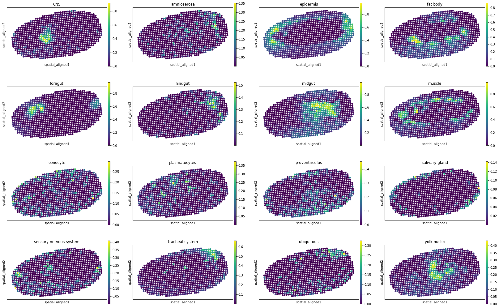
Visualizing results in 2D

for i, adata_st_i in enumerate(result):
    print("Slice %d" % (i+1))
    sc.pl.spatial(adata_st_i, img_key="hires", basis="spatial_aligned", color=model.celltypes, spot_size=1.)

Slice 1

Slice 2

Slice 3

Slice 4

Slice 5

Slice 6

Slice 7

Slice 8

Slice 9

Slice 10

Slice 11

Slice 12

Slice 13